A Simple Introduction to The Random Forest Method
Intuition, Motivation, and How it works on the Random Forest Method

1. Introduction
Random Forest lives up to its name : simply, made up of several trees. In more details, Random Forest is a set of decision trees built on random samples with different policies for splitting a node [1]. The implementation, random forest uses the bootstrap method in building decision trees and there are two ways to interpret these results; the more common approach is based on a majority vote in classification case and an average in regression case.
Related Fundamental knowledge
The ideas behind Random Forest. in fact, are containing so many topics that need to be concerned as following :
Having some basic knowledge above would help for gaining basic ideas behind Random Forest. We will discuss the bagging method first, since bagging is important part besides decision tree.
2. Bagging Method
In wikipedia — Bootstrap aggregating, also called bagging (from bootstrap aggregating), is a machine learning ensemble meta-algorithm designed to improve the stability and accuracy of machine learning algorithms used in statistical classification and regression. It also reduces variance and helps to avoid overfitting [2].
Sometimes, decision trees have a high variance since in training process data is split into two parts, fit to both halves and lead to overfitting. When predicted with new data, the predicted results can be very different. Bagging overcomes this problem by reducing variance and helps to avoid overfitting.
as explained before in the bootstrap method, bagging processes only in step Further Inference-average the population parameters as following :
- given a population with sample size n
- set of B-bootstrap sample size of n — Create a random sample with replacement from the original sample with sample size N as the original sample, replicate B time, and there will totally B Bootstrap Samples
- set of B-bootstrap estimate variance
- further inference — evaluate mean variance with sum variance in B set bootstrap divided number of B
In other words, averaging a set of B-bootstrap reduces variance. Mathematically, we can write the above process as following

This is not practical because we generally do not have access to multiple training sets. Instead, we can bootstrap, by taking repeated samples from the (single) training data set. In this approach we generate B different bootstrapped training data sets, and finally average all the predictions, to obtain

This is called bagging [3].
2.1 Out-of-Bag Error Estimation
Implementation of a method we should estimate an error, how to estimate error when implementing bagging? There is a straightforward way to estimate the test error of a bagged model without cross-validation or the validation set approach. keep in mind implementing bagging repeatedly, there are subsets of each observation (B-bootstrap) and each bagged tree makes use of around 2/3 (two-thirds) of population data. The remaining 1/3 (one-third) population data not used to fit a given bagged tree are referred to as the out-of-bag (OOB) observations.

As we discussed, in order to predict single data, we can majority vote in the classification case and average in the regression case.
3. Random Forest Method
As mentioned in the beginning, Random Forest uses the bootstrap method in building decision trees, which provide an improvement over bagged trees by way of a small tweak that decorates the trees. when building these decision trees, each time a split in a tree is considered, a random sample of m predictors is chosen as split candidates from the full set of p predictors. A fresh sample of m predictors is taken at each split, and typically we choose m ≈ √p — that is, the number of predictors considered at each split is approximately equal
to the square root of the total number of predictors [3].
In splitting process, random forest is not even allowed to consider a majority of the available predictors. Suppose that splitting process consider a strong predictor, consequently all of the bagged trees will look quite similar to each other and the predictors from the bagged trees will be highly correlated. This state is not lead to reduction variance.
Of 2 paragraphs above we can analysis, random forest
- forcing each split to consider only a subset of the predictors
- therefore, on average (p − m)/p of the splits will not even consider the strong predictor, and so other predictors will have more of a chance
Using a small value of m in building a random forest will typically be helpful when we have a large number of correlated predictors

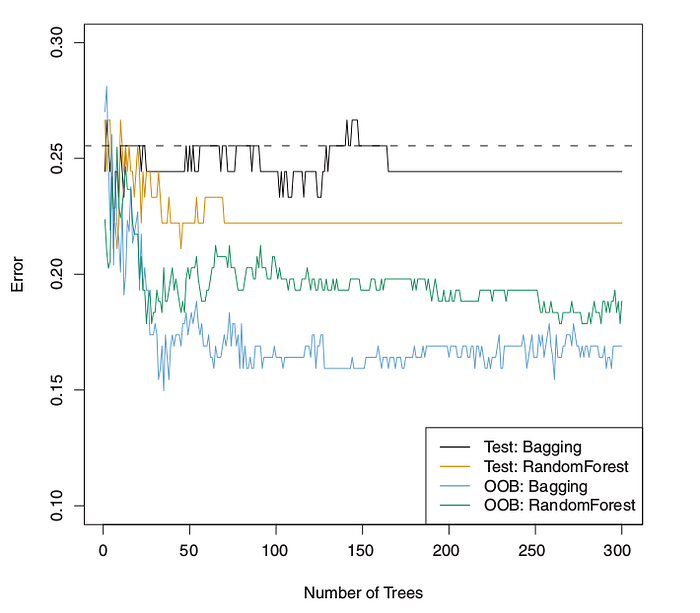
Results from random forests for the 15-class gene expression data set with p=500 predictors. The test error is displayed as a function of the number of trees. Each colored line corresponds to a different value of m, the number of predictors available for splitting at each interior tree node. Random forests (m<p) lead to a slight improvement over bagging (m=p). A single classification tree has an error rate of 45.7 % [3]
3.1 How Does Random Forest Work?
This simulation uses a “dummy” data set as follow

Step by step and intuition build random forest
1. Draw a random bootstrap sample of size m :
in order to create bootstrap data set that is the same size as original/population. we just randomly choose m samples from the original data set with replacement
this simulation, will create 3 bootstrap data set. The important detail is that we are allowed to select the same sample more than once

2. Grow a decision tree from the bootstrap sample :
- Randomly select d features without replacement.
- Split the node using the feature that provides the best split according to the objective function, for instance, by maximizing the information gain.
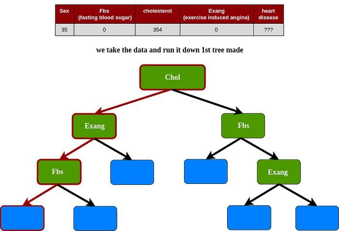
1st bootstrap data set, for the root we select randomly 2 variables as candidates : cholesterol and sex. For instance, we select cholesterol as a root, since sex has been chosen, sex not allowed as a data set. In this case we use cholesterol, Fbs, and Exang as variables.

2nd bootstrap data set, for the root we select randomly 2 variables as candidates : Fbs and sex. For instance, we select sex as a root, since Fbs has been chosen, Fbs not allowed as a data set. In this case we use Sex, cholesterol, and Exang as variables.

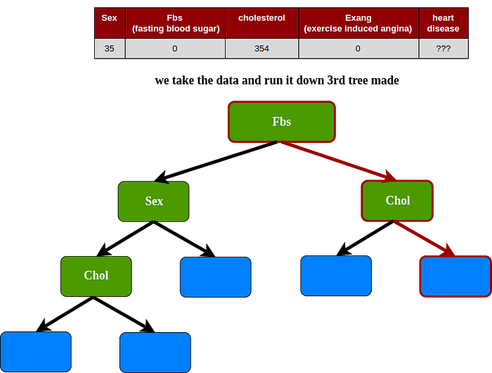
3rd bootstrap data set, for the root we select randomly 2 variables as candidates : Fbs and Exang. For instance, we select Fbs as a root, since Exang has been chosen, Exang not allowed as a data set. In this case we use Sex, cholesterol, and Fbs as variables.

3. Repeat the steps 1 to 2 k times.
4. Aggregate the prediction by each tree to assign the class label by majority vote or average.
In predict case simulation, we use a “dummy” data testing
1st tree

2nd tree

3rd tree

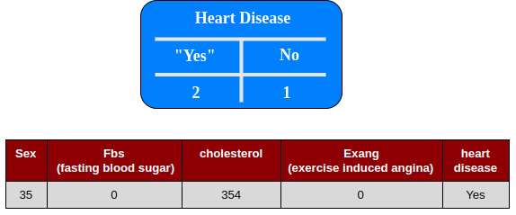
Predicting : In this case the result uses vote majority

The random forest algorithm can be summarized in four simple steps:
- Draw a random bootstrap sample of size n (randomly choose n samples from the training set with replacement).
2. Grow a decision tree from the bootstrap sample. At each node:
- Randomly select d features without replacement.
- Split the node using the feature that provides the best split according to the objective function, for instance, by maximizing the information gain.
3. Repeat the steps 1 to 2 k times.
4. Aggregate the prediction by each tree to assign the class label by majority vote or average.

Continue Learning — A Simple Introduction to The AdaBoost for Decision Tree
coming soon :)
About Me
I’m a Data Scientist, Focus on Machine Learning and Deep Learning. You can reach me from Medium and Linkedin
My Website : https://komuternak.com/
Reference
- Bonaccorso, Giuseppe. Machine Learning Algorithms. 2017
- Wikipedia — Bootstrap aggregating
- Introduction to Statistical Learning
- Raschka, Sebastian. Python Machine Learning 1st Edition
